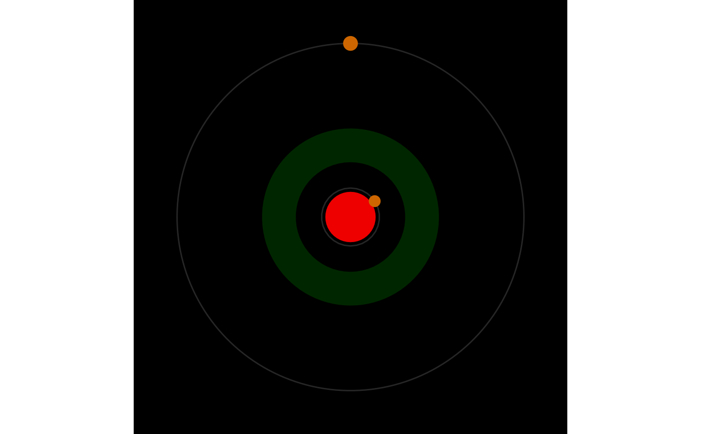
Creates a stylized polar plot of a planetary system, displaying planets in circular orbits around a central star. Planet size is scaled by radius, orbit position is randomized for aesthetics, planet color is mapped by density. The star's color is optionally based on spectral type. Optionally, star's habitable zone visualization can be overlayed.
Usage
plot_star_system(
  planet_data,
  spectral_type = " ",
  habitable_zone = c(0, 0),
  show_legend = FALSE
)
Arguments
- planet_data
A data frame containing planetary system data. Must include:
pl_orbsmax: semi-major axis (orbital distance),pl_rade: planetary radius (in Earth radii),pl_dens: planetary density (g/cm³).
- spectral_type
Optional character string indicating the star's spectral type. Accepted values:
O,B,A,F,G,K,M.- habitable_zone
Optional numeric vector containing 2 values: Inner and outer habitable zone edges in AU.
- show_legend
Optional bool value, whether to show plot legend.
Details
The central star is positioned at the origin with planets arranged in orbits of increasing radius. Orbit lines are shown in gray for clarity.
Examples
# Plot system GJ 682 (with hostid == "2.101289")
data = closest_50_exoplanets |>
  subset(hostid == 2.101289)
spectral_type = classify_star_spectral_type(data$st_teff[1])
plot_star_system(data,
                 spectral_type,
                 habitable_zone = calculate_star_habitable_zone(data$st_lum[1]))